Some ways that we can model causal effects using machine learning, statistics and econometrics, from a sixth-century religious text to the causal machine learning of 2021 including causal natural language processing.
Imagine you receive a dataset of school students and their study pathways over time, and you wish to find out whether a career coaching intervention makes a student more or less likely to go to university.
You analyse the dataset and can see some correlations. Perhaps certain subsets of students go to university after receiving an intervention, and some groups appear to be less likely to go to university when they have received the intervention.
The snag is, students who were interested in coaching may well have been interested in going to university anyway. Or perhaps the school provided career coaching only to students at risk of dropping out of education, perhaps to those students from lower-income backgrounds?
For either of these possibilities, the student’s interest, aptitude, or socioeconomic status influenced the odds of receiving career coaching, and also influences the chances of going to university. This kind of external factor is referred to as a “confounder”. How can you identify whether the career coaching influenced a student’s choice to go to university when there is a confounding factor that influences both the choice to take career coaching, and the likelihood of choosing to go to university?
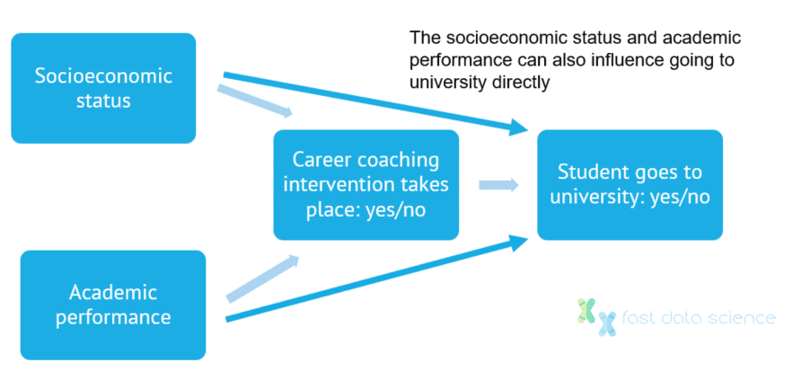
Factors such as socioeconomic status and academic performance can influence the choice to deliver an intervention, but can also directly influence the effectiveness of the intervention. How can we untangle this to discover causal relationships between the intervention and the final outcome?
Even given a large, clean, and otherwise ideal dataset, it can be very difficult to identify causal effects. Causal inference is fraught with difficulty.
Traditional machine learning techniques are based around identifying correlations and predicting outcomes based on patterns in past data. For example, a very simple machine learning model, such as a logistic regression model, can be trained to predict the probability that a hypothetical student will go to university, given information on whether or not they received an intervention. But if the intervention is tied up with that student’s aptitude and socioeconomic background, the machine learning model may not be telling us very much.
If you use either traditional non-causal machine learning or statistics, you may even find strange effects, such as the following:
This effect is surprisingly common and known as Simpson’s Paradox. Models that do not take into account causality are susceptible to this kind of misinterpretation of data.
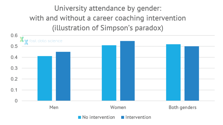
An example of Simpson’s paradox: an intervention may appear to have a negative effect when we look at both genders together, but when looking at each gender in isolation, the intervention has a positive effect.
If you increase the number of career coaching interventions passed to the model, it will simulate a hypothetical student who received more interventions, but implicitly that fictitious student now comes from a different socioeconomic background and was already more or less likely to attend university even before the intervention took place!
Whether we just look at a graph of our data, pore through numbers, or build a machine learning model, the outcome will be the same: we do not know to what extent a difference in student outcomes is due to an intervention and to what extent it is due to the student’s background.
Other analogous examples of the above problem include:
We would like to find out whether a medical treatment resulted in recovery over a dataset of a few thousand patients. However, patients who opt for the treatment tend to be in worse condition than those who don’t.
In this case, the patient’s initial state of health is a confounder. If we just look at the cohorts of patients with and without the treatment, those without the treatment will appear to have recovered better, creating the illusion that the treatment was harmful rather than beneficial.
Below you can test out a real-life example of Simpson’s Paradox from a study conducted on kidney stones in London in 1986[14]. The researchers wanted to find out which of two treatments for kidney stones had a better recovery rate. The paradox is that treatment B appears to be more effective when we look at both sizes of kidney stones together, while treatment A has a better recovery rate when we look at either size in isolation. By adjusting the numbers, you can change the ratio and find out what kind of figures make Simpson’s Paradox appear or disappear.
When the probability of an intervention being given (career coaching, medical treatment) is influenced by confounding factors outside our control, there are a number of statistical techniques from several disciplines to account for the confounders.
However, the only sure-fire way to eliminate confounders is the “gold standard” used in the pharmaceutical industry, which is the randomised controlled trial. A pharma company wants to know whether drug A is better than drug B. If they allow patients to choose which they receive, they leave themselves open to the effect of confounding factors. However, if you roll a dice and assign patients at random to either treatment, then you can compare the two cohorts A and B and know that any difference in outcomes is solely due to the treatment provided, provided the two groups are large enough.
To run a randomised controlled trial in any field, whether we are talking about pharmaceuticals, career coaching, or any other area, requires an ideal and often unobtainable situation:
In real life, we often find ourselves presented with a dataset that has already been collected (such as the data on school students mentioned above), or we can watch events unfold as an observer but cannot intervene: we cannot assign treatments.
For these tricky but very common situations, researchers across disciplines have devised a number of statistical tricks to remove or account for confounding factors and aim to discover causal relationships. However, I should emphasise that the randomised controlled trial trumps all of these techniques.
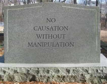
Donald Rubin and I once made up the motto
NO CAUSATION WITHOUT MANIPULATION
to emphasize the importance of this restrictionPaul Holland, influential statistician, in a 1986 paper[7]
A simple and not very sophisticated way that we may be able to remove the effect of a confounder is to segment the data. For the example of the student’s academic outcomes, we could run separate analyses, or even just plot graphs, for students in different economic and academic groups and try to identify if career coaching interventions are correlated with university attendance for students from deprived backgrounds with high grades at school.
The problem with this approach is that the segmented datasets may be too small to conduct a meaningful analysis, and this is hard to do when the confounding variable is continuous rather than discrete. Furthermore, you lose the statistical power that you would achieve with the larger complete dataset.
You also need to know about the confounder and have data on it in order to segment on it, so we can’t segment when the confounder is unknown (if we have no data on whether students in our dataset come from single-parents or nuclear families, we cannot segment on this in order to remove it as a confounder).
Fast Data Science - London
Another approach to remove confounders is to take every student who received an intervention, and match them to a student from a similar financial and school grade background who did not receive the intervention. There are a number of statistical techniques that allow us to calculate matches, such as propensity score matching. However, matching can be labour intensive, inflexible, and can actually amplify bias due to confounding factors.
In certain fields such as economics, sociology, or policy analysis, it is rare that a researcher has a chance to do a proper experimental study like a randomised controlled trial. Since the 1930s, researchers in the social sciences have had to use statistical methods to try to identify causality.
If there is a factor that influences the assignment of an intervention which you believe to be partly random or not subject to bias, you can pretend that you have run a randomised controlled trial. An experiment like this in the absence of a true intervention is called a quasi-experiment.
A particular kind of quasi-experiment that has been used since the 1930s but which became popular in econometrics in the 1980s is instrumental variables estimation.
In the example of our career coaching intervention, let us imagine that we have a dataset containing not only all career coaching interventions which took place, but also those interventions which were scheduled to take place but were then cancelled due to the lockdowns (or any other factor outside the students’ control).
I don’t think that there would be any difference in terms of motivation or socioeconomic background between two students whose career coaching sessions were scheduled a week apart, one before and one after 26 March 2020 (the date of the first lockdown in England).
The cancellation or non-cancellation of a careers session is therefore a variable that is uncorrelated with our confounding factors. This is called our instrumental variable.
The instrumental variable gives us a way in to compare two students where we know that the intervention was at least partly influenced by the quasi-random factor which we are aware of.
An instrumental variable must have a direct effect on the independent variable in a quasi-experiment, but no direct effect on the dependent variable.
Some very good candidates for instrumental variables that can help you run a quasi-experiment are effects that originate from:
Our instrumental variable must be a value that influences whether the student participated in a careers advice session, but which does not directly influence their choice to go to university.

Our instrumental variable must influence whether an intervention is given, but cannot directly influence the outcome.
The student’s socioeconomic background is not a good candidate for an instrumental variable because it directly affects the student’s chances of going to university, with or without the careers coaching.

We can’t use socioeconomic background as an instrument because it also has a direct influence on university choices regardless of the intervention.
The Covid lockdown does presumably affect a student’s chances of going to university, but I would imagine that if you took a dataset of students with scheduled appointments in March 2020, then the date of the careers falling inside or outside the lockdown dates would be as good as random.
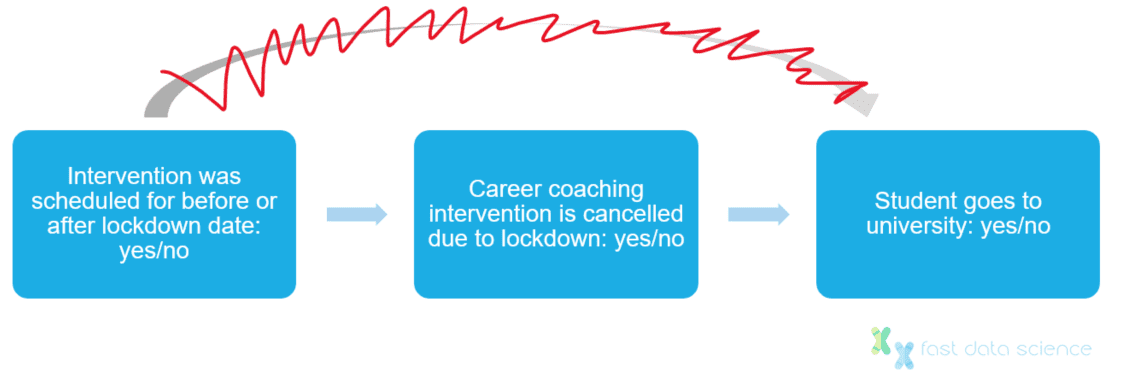
We can assume that an intervention scheduled for March 2020 would be cancelled if it fell under a lockdown. This effect is unrelated to student’s academic ability or finances, and would not influence university attendance directly.
Interventions falling under lockdown is therefore a suitable instrumental variable.

The Babylonian Talmud was written in the sixth century and limited school class sizes to 40 students. Image source: Wikimedia.
וְאָמַר רָבָא סַךְ מַקְרֵי דַרְדְּקֵי עֶשְׂרִין וְחַמְשָׁה יָנוֹקֵי וְאִי אִיכָּא חַמְשִׁין מוֹתְבִינַן תְּרֵי וְאִי אִיכָּא אַרְבְּעִין מוֹקְמִינַן רֵישׁ דּוּכְנָא וּמְסַיְּיעִין לֵיהּ מִמָּתָא
And Rava said: The maximum number of students for one teacher of children is twenty-five children. And if there are fifty children in a single place, one establishes two teachers, so that each one teaches twenty-five students. And if there are forty children, one establishes an assistant, and the teacher receives help from the residents of the town to pay the salary of the assistant.Bava Batra (“The Last Gate”), Babylonian Talmud (Jewish sacred text completed in 6th Century AD)
Maimonides was a Jewish scholar who lived in Spain in the 12th Century. He interpreted the above quote from the Babylonian Talmud as an instruction to limit all school class sizes to 40 students.
According to Maimonides’ rule, any class which exceeds 40 students must be split, so a cohort of 41 students would become a class of 20 and another class of 21 students. The class limit of 40 students became law in modern Israel.
In 1999, the economists Joshua Angrist and Victor Lavy wanted to measure the effect of class size on Israeli children’s reading levels, but faced the confounding factor that class sizes are correlated with socioeconomic groups. More affluent parents tend to have the option of sending their children to schools with better teacher-to-pupil ratios.
Clearly, no parent would consent to their child participating in a randomised controlled trial of different class sizes. So Angrist and Lavy were limited to an observational (non-interventional) study but faced a challenge of how to separate the causal effect of the class size on the learning outcome, from the causal effect of the parents’ background on the learning outcome, when the parents’ background and the class size were themselves correlated.
Angrist and Lavy’s workaround was to take all classes of size 40, 20 and 21, and assume that class sizes around these values are random, since nobody can predict whether 40 or 41 children will be enrolled in a particular year. They were therefore able to compare the reading comprehension scores of children in very small and very large classes, knowing that the class size itself was independent of the parents’ economic and educational background and other confounding factors.
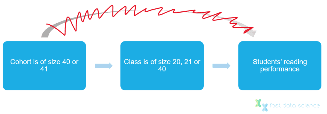
Cohort sizes around the legal threshold of 40 are unrelated to parent’s socioeconomic background, do not directly influence learning outcomes, and can therefore be used as an instrumental variable.
Using this clever trick, Angrist and Lavy were able to leverage the side effects of an administrative rule and conduct an analysis almost as if they had run a randomised controlled trial. This is an elegant example of how causality can sometimes be inferred even if the researcher is not able to conduct an experiment.
Joshua Angrist worked on another paper where he investigated the effect of serving in the Vietnam War on lifetime earnings. Here, he encountered a similar problem: people with higher education levels are less likely to enrol in the military voluntarily, and also tend to have high average earnings whether or not they serve in the military.
Fortunately, the US government ran a series of draft lotteries, where men were enlisted to fight in the war by a random process: an ideal candidate for an instrumental variable. By knowing the proportion of voluntary recruits, conscientious objectors and people rejected on medical grounds, Angrist was able to estimate a 15% drop in earnings for white veterans compared to nonveterans.
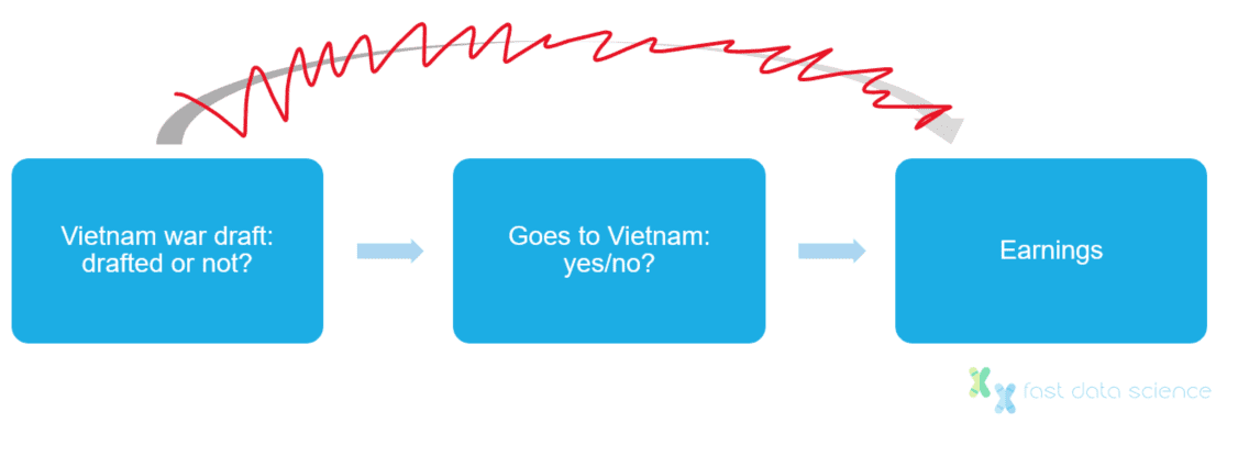
The draft lottery is random and only has a direct influence on whether an individual goes to Vietnam or not, but has no direct influence on earnings. Therefore the draft could be used as an instrumental variable to remove the confounding factor that highly educated people do not tend to enlist in the military.
The approaches I have described above are mostly from the fields of statistics and economics. However, machine learning as a field has generally been non-causal and deals with cleverer and smarter associations or correlations between things. For example, a state of the art neural network can classify images into different dog breeds, or predict what a customer is about to spend, but does not attempt to address the why: what it is that causes a customer to spend more or less.
There have been a number of attempts over the years to develop causal machine learning models, or introduce causality into existing frameworks. A lot of causal AI mechanisms involve creating a graph showing how events cause each other. One of the best-known frameworks is Bayesian networks:
The computer scientist Judea Pearl developed a sophisticated way of representing causal relationships in a directed graph called a Bayesian network.[11] Arrows are drawn when a causal relationship exists between two nodes of the graph, although the statistical correlation observed will not depend on the direction of the arrow. Bayesian networks are able to represent concepts from econometrics such as instrumental variables.
Pearl also developed the ‘do-calculus’, where a distinction is made between the probability of a student attending university given that a career coaching intervention was given:
P(student attends university | student received an intervention)
and the probability that the student attended university given that we (the experimenter) forced an intervention to be given:
P(student attends university | do(student received an intervention) )
Bayesian networks are powerful because they can represent very complex networks of relationships. They have been used in fields such as medical science to represent how symptoms and diseases are interlinked. For example the network below shows a Bayesian model for the prediction of Alzheimer’s disease.
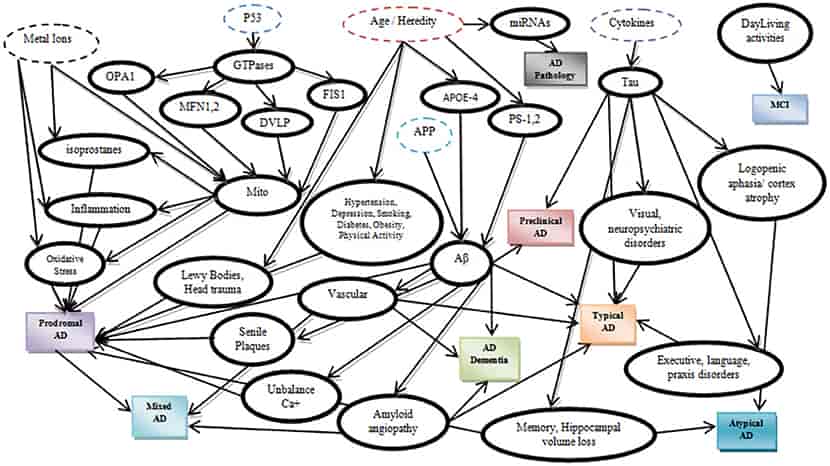
A Bayesian network which has been learned showing the causal relationships associated with Alzheimer’s disease. Image source: [1]
It is also possible for a Bayesian network structure to be learned. For example, thousands of proteins and genes co-occur in the body. It is difficult to guess the chains of cause and effect, but using statistical methods we have been able to learn the structure of Bayesian networks and guess causal relationships.
A couple of epidemiologists ran a study in 2012 investigating the causes of childhood diarrhoea in Pakistan[8]. Traditional statistics uncovered 12 variables which were associated with diarrhoea, including the number of rooms in the household. This was difficult to interpret. However, an analysis with a causal Bayesian network was able to show a network map with three variables that directly influenced the occurrence of diarrhoea: no formal garbage collection, access to a dry pit latrine, and access to an atypical other water source. The insights gained from the study could bring huge social benefit if they are incorporated into policy.
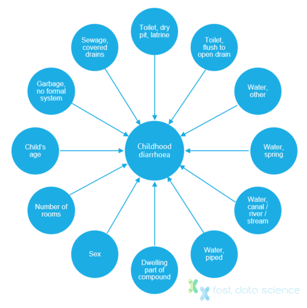
Graph showing the correlations between other factors and childhood diarrhoea incidence. Using the Bayesian network approach, the epidemiologists were able to identify three probable causal factors behind diarrhoea: no formal garbage collection, access to a dry pit latrine, and access to an atypical other water source. Image adapted from [8].
The large amount of data collected by tech giants such as Facebook and Google paved the way for the adoption of deep neural networks for purposes across industries, while in science, projects such as the 1000 Genomes Project have gathered over two hundred terabytes of information[12]. When we want to ask who to recommend somebody to connect to on a social network, or identify which gene is associated with a particular type of cancer, we can deploy cutting-edge machine learning models such as neural networks to mine associations in the data.
However, the association of a gene with cancer is not a causal question, but a statistical one. Deep neural networks are sophisticated and powerful but some of the hype around them ignores the fact that they are not usually addressing causal questions. Causal questions cannot be answered by data alone, but require a model of the processes that generate data.
For example, we can construct a model that specifies that a gene can influence a person’s susceptibility to cancer, but not vice versa. However, we would need to consider the possibility of confounders such as a mediator (the gene influences a behaviour, such as smoking, which itself increases the risk of cancer). The tools from econometrics or Bayesian networks can be adapted to this kind of model, which requires a real-world understanding of what can influence what.
In some cases, it is possible to use the time order of events in order to learn causal relationships. A student receiving a careers intervention and then attending university one year later means that the university attendance cannot influence the careers intervention. A popular method for using time series is called Granger causality, which uses the time of different events and determines which event better explains the other event.
Reinforcement learning is a field of AI that is used to learn interactions with an environment, such as a chess-playing AI or a self-driving car. An AI is considered an ‘agent’ which can take actions that result in a reward. The reinforcement learning algorithm allows the agent to sometimes take the optimal action (take the knight) but sometimes to ’explore’ (take a lower value piece) with an aim of learning a better strategy for the future. Although in a sense reinforcement learning is inherently causal, there have been recent modifications to reinforcement learning algorithms to incorporate the sophistication of Bayesian networks to handle confounders and other effects.
My particular field of interest is natural language processing (NLP), and I will write a little about how we can use NLP in causality.
Most NLP applications deployed in industry are used for making predictions. For example, given a jobseeker’s CV, what is that person’s most likely salary? Given an incoming email text, which department should it be forwarded to?
However, there is no reason why either the variables in a cause-and-effect scenario must be numeric. A text field could feature as a cause of a numeric field, or manifest itself as an effect, or even be used as an instrumental variable.
A predictive model to assign jobseekers to salary bands would discover a correlation between the two. But does the wording of your CV cause your salary, or are the content of the document and the salary value both a result of a common cause such as years of experience? Some degree of experimentation is possible in this area. In 2004, Marianne Bertrand and Sendhil Mullainathan sent fake CVs to employers in Boston and Chicago, randomly assigning names that sounded African-American or White, finding that the White “candidates” received 50% more callbacks for interviews.[5] However, if a causal model can be adapted to text fields, we can learn from observational data instead of needing to conduct interventions.
An example case where we would like to understand causality, where the cause is a text field, without conducting an experiment, is as follows:
Users post comments on an online forum. Every user has a gender icon on their profile: ♂ or ♀. Users labelled ♀ tend to receive fewer likes. Are the fewer likes due to the icon, or due to the content of the text?[6]
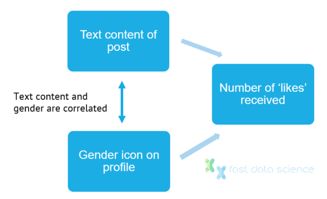
It is hard to separate out the effects of the profile icon from any property of the text content, both of which are influenced by the user’s gender. Causal machine learning techniques can generalise the ideas behind instrumental variables to remove the confounding factors.
There are a number of solutions to this kind of problem.
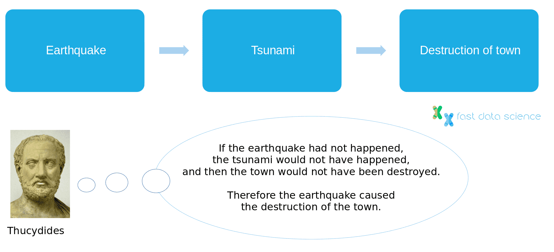
I recommend reading The Book of Why[12] by Judea Pearl, which delves into causality from many angles. One of the interesting points that Pearl makes is that throughout history, we have not always had a clear-cut definition of causality. For example, the Greek historian Thucydides described an incident where an earthquake caused a tsunami which itself destroyed a town in 426 BC. Thucydides concluded that the earthquake had been the ultimate cause of the destruction of the town because
ἄνευ δὲ σεισμοῦ οὐκ ἄν μοι δοκεῖ τὸ τοιοῦτο ξυμβῆναι γενέσθαι….
without an earthquake I do not see how such an accident could happen.
History of the Peloponnesian War, Thucydides, early fourth century BC[14]
This is one definition of a cause: we imagine a parallel universe where the first event did not take place, and imagine what would have been the consequence. The imagined ‘what-if’ scenario is called a counterfactual.
Curiously, many centuries later the Scottish philosopher David Hume defined causality as the association between two events which regularly occur in succession. So we infer that a flame causes heat, because every time we see a flame, we feel heat on touching it. This is called the regularity definition of causation.
Nine years later, Hume revised his definition of causation from the regularity definition back to the counterfactual definition, stating that we can infer causation where
if the first object had not been, the second had never existed
David Hume, Enquiry Concerning Human Understanding[16]
So after further thought, Hume settled on Thucydides’ definition of causality. Today the most widely accepted definition of causation is the counterfactual definition, although it raises many other questions (do we imagine a universe where one event didn’t happen, but everything else was identical? Which universe do we choose if there are multiple candidates?).
After reading about the counterfactual definition of causality, I wondered why many European languages use different verb forms to differentiate events that definitely didn’t happen from events that really happened, or may have happened. For example, in Spanish a ‘what-if’ conditional statement for a counterfactual scenario is formed using the formula
si (‘if’) + imperfect subjunctive verb + conditional tense
for example, si no hubiera llovido, no me habría mojado (‘if it had not rained, I would not have got wet’), where hubiera is the imperfect subjunctive form of the verb, signifying a scenario that didn’t happen. If the speaker considers it likely or possible that it did rain, they would say si ha llovido using ha in place of hubiera.
In English we tend to use the past tense with had for an event that didn’t happen (counterfactuals) and other forms such as the past tense with have for events that did happen:
‘if’ + past tense with had + conditional tense with would have
So we have if it had not rained, I would not have got wet (rain did not happen) as opposed to if it hasn’t rained, I won’t get wet (rain may have happened). Another example of this distinction is the use of were in phrases like if I were you, or if he were rich - the choice of were rather than was in these sentences indicates to the listener that we are imagining a world where somebody is rich, who is not rich in our world.
German, French and Italian also have subjunctive verb forms, while Chinese uses different particles in the sentence to distinguish counterfactual and non-counterfactual conditions[15], although the definition of which hypothetical scenarios require special verb forms varies subtly across languages - not all Spanish subjunctive sentences require a subjunctive in Italian, and vice versa. In Chinese the counterfactual grammatical particles are mostly optional.
The fact that counterfactuals are baked into the grammar of our languages is interesting as it shows that although causality can be hard for us to understand (if causation were easy to understand, then Simpson’s Paradox would not be a paradox!), it is an intrinsic part of how we think and communicate.
Children by the age of 6 to 8 are usually able to master the tenses in their native language. For me, this implies that even small children are able to understand and grasp counterfactuals intuitively. In 2019 Keito Nakamichi did an experiment to investigate just this, and found that four to six-year-olds are able to think about counterfactuals associated with emotional events but not physical events.[17]
I tried a very non-scientific experiment on my six-year-olds and I found that they could accurately answer counterfactuals but didn’t use the were/would syntax effectively, and sometimes used will instead. They formed ungrammatical sentences such as *if James’s parents didn’t die, he will live with them by the seaside, showing that they understood the counterfactuals but hadn’t mastered the conditional and subjunctive verb forms.
Causality models are becoming widespread and data scientists are beginning to need a basic understanding of causality theory. Traditional machine learning models are focused on correlation, but for cases like the example of the students receiving a careers advice intervention, a machine learning or statistical approach which ignores causality will deliver misleading results, such as the impression that a careers intervention has a detrimental effect on a student attending university. Clearly, if the interventions themselves were targeted at students who were at risk of dropping out of education, this conclusion would be nonsensical.
There are two schools of thought for causal models: the older methods from econometrics and the social sciences, and the newer models coming from computer science such as Bayesian networks. However any causal model cannot be purely data-driven, but must be designed to incorporate its creator’s understanding of the causal mechanisms in place, such as Vietnam war draft ➜ enlistment in army ➜ lifetime earnings.
Causality models have been used in the social sciences since at least the 1930s, while natural language processing has become widespread in industry, in particular in the last decade or so, due to advances in dataset size and computing power. Researchers and industry leaders are only recently beginning to ask how causality and NLP can be combined. The recent breakthroughs in ever more sophisticated vector representations of text and proliferation of easily accessible text datasets mean that we can expect to see more discussion of NLP and causality in the near future.
Unleash the potential of your NLP projects with the right talent. Post your job with us and attract candidates who are as passionate about natural language processing.
Hire NLP Experts
Unlock your business potential with expert AI consulting services from Fast Data Science. Discover strategies to accelerate growth and outperform competitors.

Financial advisors, like lawyers, are regulated in the UK. All financial advisors should be registered with the Financial Conduct Authority (FCA) and must have certain qualifications and have signed up to a code of ethics. UK financial advisors must also complete professional training every year.
What we can do for you