I’ve put together a short selection of some intermediate-level data science concepts which give you a good grounding in the field. A lot of these are based on a series of articles which I wrote for the excellent data science resource deepai.org. I’ve biased the list of data science concepts a bit towards natural language processing, because that’s the area I mainly work in.
An Activation Function is used in neural networks and acts as a ‘gatekeeper’. It lets large signals through, but blocks small signals.
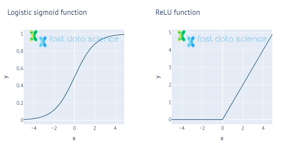
Two of the commonest activation functions, the logistic sigmoid function and the ReLU function. All activation functions output a small value for small x, and a large value for large x, and are non-linear.
Activation functions were inspired by the action potential, which is a blocking function in biological neural networks.

Two British scientists, Hodgkin and Huxley, discovered action potentials in living creatures by dissecting the nerves of a squid. This later served as the inspiration for the activation potentials used in neural networks.
Without activation functions, neural networks would not be able to recognise objects and faces. In fact they would be no better than a simple regression model such as the line-of-best-fit in Excel.
A common choice of activation function is the Sigmoid Function.
Backpropagation is a technique for efficiently calculating weights inside deep neural networks. It involves calculating the loss function at the end of the network, and then walking back towards the beginning of the network and updating the network weights.
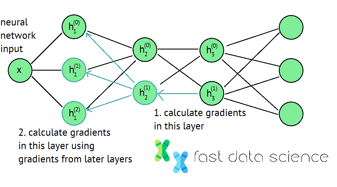
The backpropagation algorithm is key to deep learning and data science. It involves working your way backwards through a neural network from its end to its start, at each point calculating how you need to update the weights. Read in more details here.
Convolutional Neural Networks are a special kind of deep neural network which is mainly used for recognising images. They have a rigid structure that allows them to recognise patterns inside an image, as well as combinations of patterns.
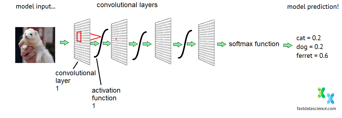
Schematic diagram of the architecture of a convolutional neural network. Normally networks that process photos or faces have at least 20 layers.
Interestingly, convolutional neural networks aren’t useful only for images. They can be repurposed for sound signals (you can take any sound recording and convert it to a spectrogram, and then it behaves like an image). You can also take a document in English or another language, and convert it to an image-like form by replacing each word by its a word vector embedding.
Deep Learning is a kind of machine learning technique that involves layering many simpler machine learning models on top of each other, and gluing them together with an Activation Function. The rise of deep learning has enabled much of the advanced AI that we see today, from machine translation to Snapchat filters.
Convolutional neural networks, as described above, are a kind of deep learning model.
Traditional machine learning models involve a much smaller number of parameters, and often end up doing only a few simple operations on some incoming numbers. In contrast, with deep learning, a number is input (such as a pixel or fragment of audio signal), and it passes through many layers of mathematical operations before the model produces its output:
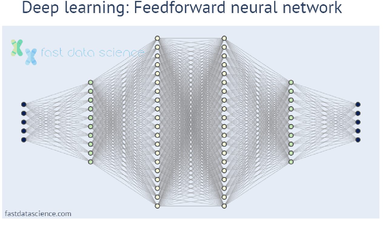
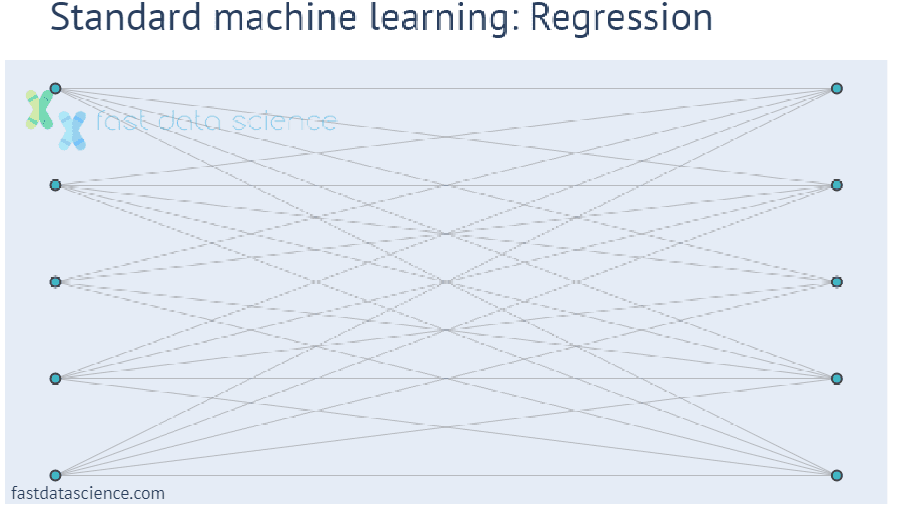
Unfortunately, deep learning models are becoming ever more complex and hard for humans to understand, creating a need for explainable AI and explainable machine learning models.
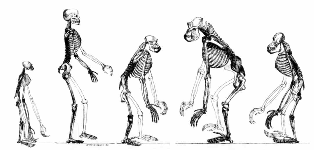
An Evolutionary Algorithm is way of improving an AI using methods inspired by biological evolution, in particular random mutations and natural selection.
If you train a machine learning model, it can be tempting to measure its performance using accuracy. For example, if a model to identify presence/absence of tumours scores 90% accuracy, that’s good, right? But what if 90% of your patients have no tumour, and the model predicts ’no tumour’ for 100% of your patients? The model is completely useless but would still score 90%! That’s why we use the F-Score, which is a more robust measure and key data science concept that can handle imbalanced classes.

Definition of the F-score in terms of precision and recall

Definition of precision and recall in terms of true positives (tp), false positives (fp) and false negatives (fn)
In fact, if somebody tries to get you to invest in a data science model and they will only tell you a figure such as ‘90% accuracy’, you should be quite suspicious! They could well be dealing with a problem of data imbalance, where 90% accuracy is very easy to achieve. The F-score is more robust against this kind of effect.

A synthetic face generated by a generative adversarial network
Generative Adversarial Networks are a clever neural network design, where we put two neural networks together and pit them against each other (hence the ‘adversarial’ in the name). One network is given a task to generate things (such as face images), and the other network’s task is to distinguish what was generated from the real thing (so it must learn to tell fake faces from real faces). Over time this adversarial set-up gives us a very sophisticated generator which can create life-like face images, music, artwork, videos and even text.
Hyperparameter optimisation is the process of choosing the best hyperparameters, or learning parameters, for a machine learning algorithm. For example, if you are building a face recogniser with a neural network, you might want to experiment with different learning rates, numbers of layers, learning algorithms, image dimensions, and so on. Since each time you train a model could take months, it is not practical to experiment with every possible combination of hyperparameters, and so it’s common to use clever algorithms that converge towards the best values quickly.
When we are training a decision tree, information gain is the reduction in entropy, or surprise, that we obtain by splitting our dataset on a certain value of a variable.
For example, if we want to decide whether to add a branch to a decision tree with threshold age > 50, we would work out if this cutoff results in two datasets that are each more homogenous than the original dataset. The change in entropy corresponds to the information gain.
The Jaccard Similarity Index is a number that tells us how similar two documents are to each other. It can be a percentage or a number between 0 and 1.
Imagine that you want to measure out how similar these two sentences are:
Document A: ’learning data science is easy’
Document B: ‘it is easy to become a data scientist’
I’ve marked in bold the words that occur in both sentences.
Regardless of whether we agree with the statements, we can use the Jaccard Similarity Index formula to calculate how similar Document A is to Document B:

Mathematical definition of the Jaccard Similarity Index
So for our two sentences, there are two words in common, and a total of ten words altogether. We can visualise the calculation in a Venn diagram:
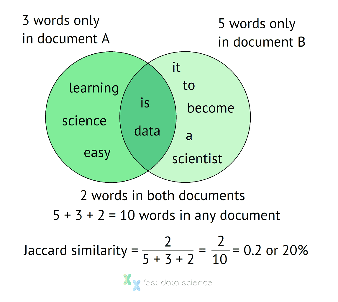
Venn diagram of how to calculate the Jaccard Similarity Index for two sentences. The sentences have 10 words in total without double counting, and two words occur in both documents, giving us a Jaccard Similarity Index of 20%.
From the Venn diagram it’s easy to see that the two documents have a Jaccard Similarity of 20%, that is, they are 20% similar to each other. If no words were shared between the documents, then the similarity would come to 0.
Because it’s debatable that ‘science’ and ‘scientist’ are somewhat similar, sometimes we can use the Jaccard index on sub-word level. For example, we might take sequences of three letters called trigrams: ‘sci’, ‘cie’, ‘ien’, ’ent’, ’nti’, ’tis’, ‘ist’ - with this measure, ‘science’ and ‘scientist’ have a similarity of 33%.
There are a number of alternatives to the Jaccard Index, such as the Cosine Similarity Index.
K-means clustering is an extremely simple algorithm for clustering, or discovering groups and topics in a dataset. For example, imagine you have 100 news articles about various topics. You can use the K-means clustering algorithm to discover that there are 5 topics in the dataset: sport, politics, technology, world, and business. K-means works for all kinds of data, not just text. For example, companies can group their customers into strata based on preferences and spending patterns.
Fast Data Science - London

Animation showing how the k-means algorithm works. Initially the cluster centres are randomly chosen. Then we alternate between assigning every data point to its nearest cluster, and then re-calculating the centre of every cluster according to all its datapoints, until the cluster assignments stop changing.
Latent Dirichlet Allocation (LDA) is an algorithm used in natural language processing for clustering text documents. LDA is more sophisticated than K-means, and can assign documents to multiple categories each with a probability.
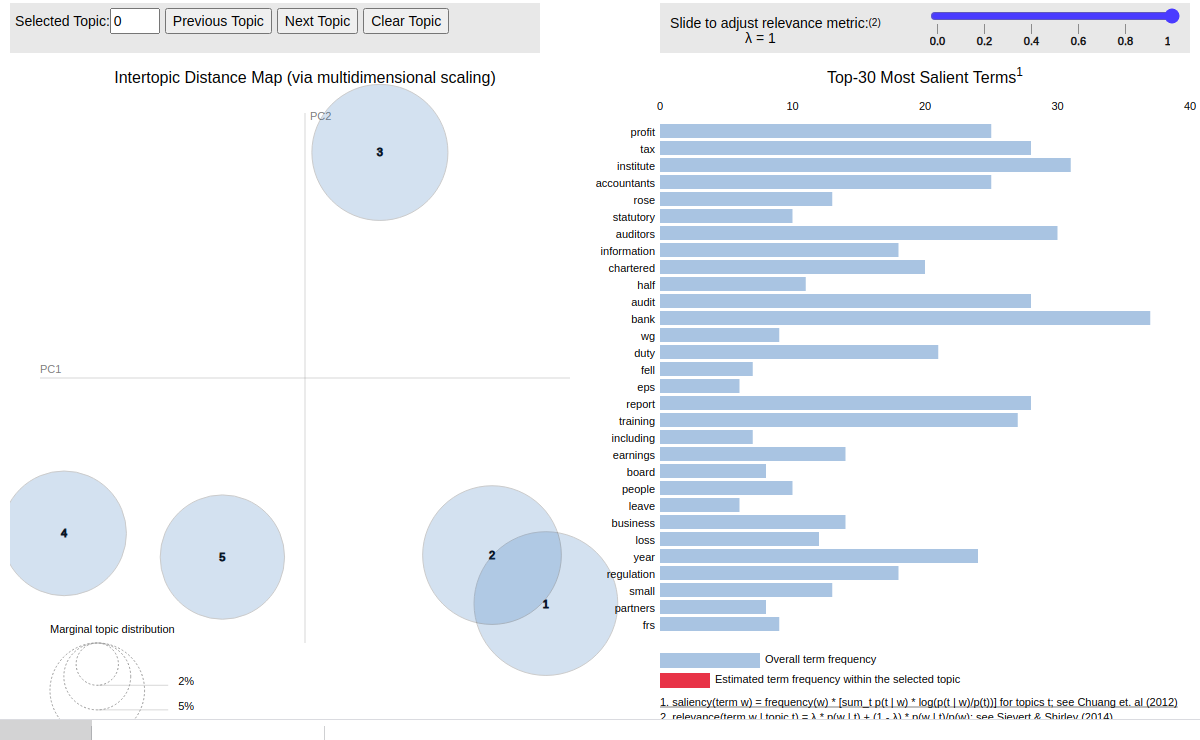
Visualisation of clusters assigned by Latent Dirichlet Analysis, using text from the British National Corpus (BNC). The clustering algorithm also outputs weights for words in the corpus, allowing us to easily assign any new incoming document to a cluster.
A Markov Chain is a simple model used to define the state of a system as a node in a graph. For example, a lift (elevator) has three states: stopped, going up, and going down. A Markov Chain could be designed to represent these three states as nodes on a graph with transition probabilities representing how likely the system is to switch from one state to another.

A schematic of what a Markov chain could look like for a lift/elevator. There are three states, and numbers on the transitions indicate the probabilities.
Many machine learning models, in particular models for speech and handwriting recognition, are based on Hidden Markov Models, which are similar to the concept of the Markov Chain except that the state of the model is not visible (representing for example the word uttered in a speech recording), and we can only observe values emitted from each state (representing the data recorded in the recording).

Finally, Markov Chain Monte Carlo (MCMC) models are very powerful tools in machine learning (although very slow and hard to compute). They allow us to generate samples from an arbitrary probability distribution. This allows us to manipulate probability distributions in clever ways. For example, you can calculate a regression line on a set of data, while including a strong prior belief that the intercept is 0. This means that you can create models that combine information from training data and information from prior beliefs.
The simplest kind of text classifier you can build is a Naive Bayes Classifier. This is a basic NLP and data science concept. For example, if you want to make a spam filter, which categorises emails as spam or ham (unsolicited vs solicited mail), then the easiest tool for the job is the Naive Bayes Classifier.
The Naive Bayes clasifier is ’naive’ because it assumes that text is made up of a group of randomly occurring words, which are independent of each other. Even though this isn’t true, naive Bayes classifiers perform surprisingly well and it’s quite easy to make your own working text classifier.
Naive Bayes classifiers have the advantages of not needing much training data, making them ideal for situations where you are having to manually tag your data and your dataset is unlikely to reach a size where a neural network or large language model will bring an increase in performance.
Mathematical optimisation is a complementary technique to machine learning, and sometimes overlaps with machine learning. Optimisation is often expressed as: choosing the best option from a set of many options, which minimises a cost.
Examples of classical optimisation problems include the Travelling Salesman Problem (where a salesman must find the shortest route through all the cities on his itinerary), and the Bin-Packing Problem. where items of different sizes must be packed efficiently into a finite number of containers.
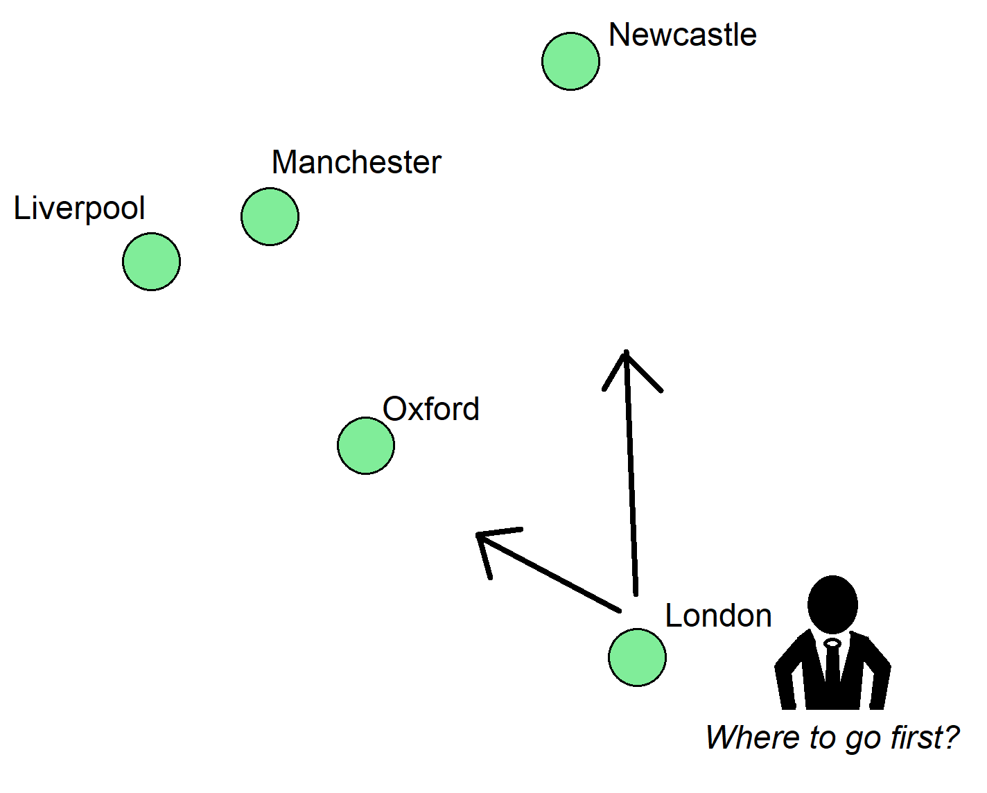
The Travelling Salesman Problem is a classic optimisation problem. Imagine our salesman has to visit these five cities. If he knows the distances between them, what’s the shortest route that stops off at every city once and only once?

Map of historical Kaliningrad, Russia. The mathematician Leonhard Euler found that it was impossible to walk over all bridges of the city and end up where he started. This is a kind of optimisation problem called a routing problem. Euler founded a new branch of mathematics, graph theory, in order to improve his Sunday stroll. Euler’s problem is famously known as the Seven Bridges of Königsberg.
Precision and Recall are two numbers which we use to evaluate the performance of a model. Their best-known use is for evaluating search engines. Precision represents how relevant the results from the search engine are, and recall represents its coverage. It is much more informative to report the performance of a model in terms of precision and recall, e.g. precision = 0.8, recall = 0.4, rather than using accuracy.

Mathematical definitions of precision and recall
Let’s imagine you work in a factory and you have a machine learning model that identifies product defects. You test the model out on ten products and find that five products were correctly identified as defective (true positive), one was misidentified as defective but was actually fine (false positive), two were correctly identified as negative (true negative) and two were actually defective but the model didn’t catch then (false negative). We can make a confusion matrix, which is a representation of how many products we got right and wrong and what kinds of errors we made:
| Really defective | Really not defective | |
| Model found defect | tp = 5 | fp = 1 |
| Model didn't find defect | fn = 2 | tn = 2 |
Confusion matrix of a machine learning model which is supposed to identify product defects
We can take the numbers from the confusion matrix and put them into the formulae for precision and recall and F-score above to get:
These three numbers are much more informative than reporting the accuracy alone.
Q-Learning is a technique in reinforcement learning which allows a robot to learn a policy, or general strategy, that it will apply to future situations. There is a reward function Q which represents the reward that the robot expects to receive for a given action.
For example, if a robot is learning to play chess, perhaps one move has Q = 0.8 and the other move has Q = 0.2, based on past games against humans. The robot would not always necessarily choose the highest Q, since sometimes it is necessary to explore other possibilities. This is called the tradeoff between exploration and exploitation.
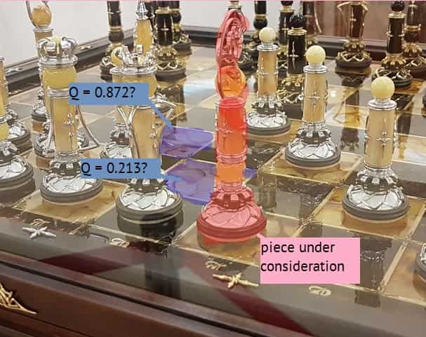
A chess-playing AI would have calculated a Q-score for each possible move it can take, but it would not necessarily always take the highest scoring move, because there is value in ’exploration’ as well as ’exploitation’.
Q-learning can be summarised as follows:
A Random Forest is a machine learning algorithm which can be used for nearly any task. Random Forests are extremely robust and good at fitting non-homogeneous data, such as tables of customer information of different data types (age, gender, credit score, past expenditure).
For this reason, Random Forests are widely used for business applications of AI. An alternative to Random Forests is a Gradient Boosted Tree.
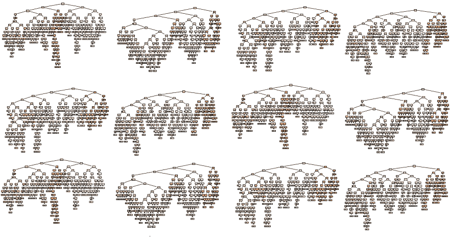
A single Random Forest model could be made up of thousands of complex and inaccurate decision trees. These trees all vote together to produce the best answer.
A Random Forest model is made up of many decision trees which have all been trained on a snapshot of the data. Each decision tree alone is not very accurate (they are ‘weak learners’), but the combination of their outputs can be very accurate. This is a bit like the classic fairground game of ‘guess the weight of the pig’, where the average guess of all participants can be surprisingly accurate.
The Sigmoid Function is a mathematical function with an S-shaped curve. The sigmoid function is used in many areas of machine learning, such as in logistic regression, where it translates a number into a probability between 0 and 1. The best-known sigmoid function is the Logistic Sigmoid function, which looks like this:
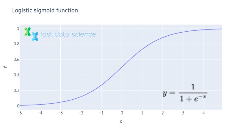
The Softmax Function is a generalisation of the sigmoid function to many dimensions. For example, if you are training a convolutional neural network to classify images into ‘cat’, ‘dog’ or ‘ferret’, the last layer would be a ‘softmax’ layer which would output three probabilities which sum to one.

A Transformer is a cutting-edge neural network design that is very useful for processing sequential data, such as text classification, machine translations, audio recordings, genome sequences, and music. A transformer neural network has a component called an attention mechanism, which allows the transformer to pay particular attention to certain words to the left and right of a particular word when processing it. The attention mechanism makes it possible, for example, to translate the word ‘it’ into the French or Spanish word of the appropriate gender by paying attention to the entire sentence.
The best-known transformer based model is BERT (Bidirectional Encoder Representations from Transformers), which was open-sourced by Google in 2018.
Most widely known machine learning algorithms are supervised learning algorithms, where a model is given a series of training examples, such as images, and a series of corresponding labels, such as ‘cat’ vs ‘dog’, and learns to label new unseen images.
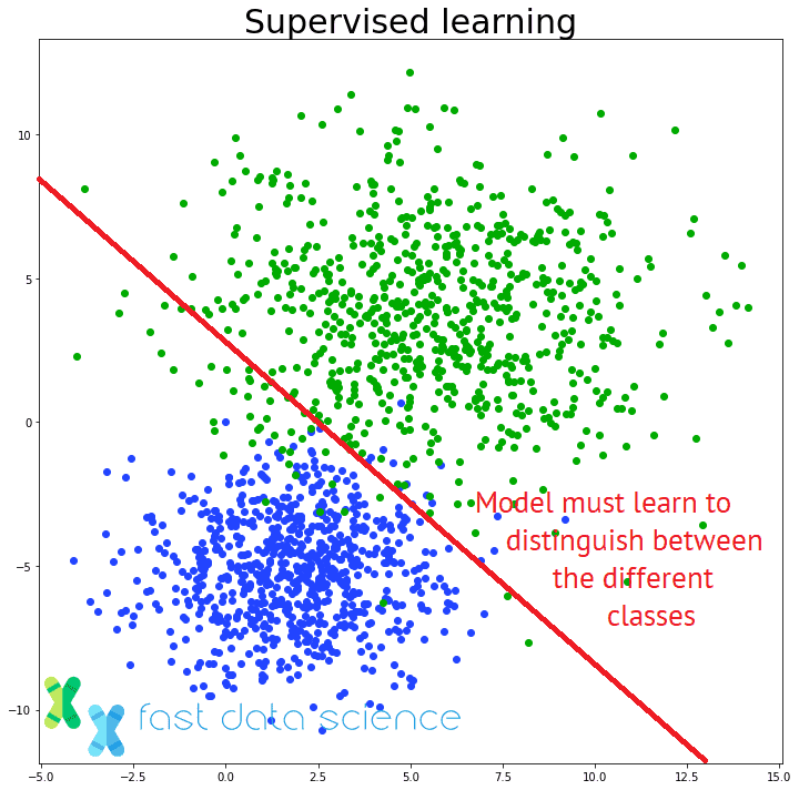
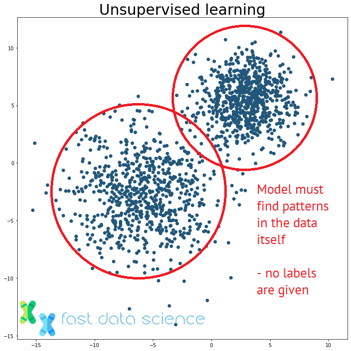
The distinction between supervised and unsupervised learning: an unsupervised learning model must find patterns in unstructured data without being told the correct answers.
Unsupervised Learning is an umbrella term for the machine learning algorithms which do not use labels, but merely look for patterns in the data. Simple examples of unsupervised learning algorithms include clustering algorithms such as k-means clustering, or Latent Dirichlet Allocation (LDA).
An example of supervised learning would be a model which classifies incoming emails for triage to the complaints or sales department, based on what a human has decided for past emails.
The equivalent problem in unsupervised learning would be: we receive a package of unclassified emails, and we have no idea if they should be grouped into two or ten groups, and we have no idea what those groups are. An unsupervised learning algorithm would have to discover clusters and topics itself.
When you are training a machine learning model, it’s important to keep a distinction usually between your training set, validation set, and test set. But what is the difference between the validation set and test set, and why do I need both?
Think of it like a student at school studying for a big exam on calculus:
When we train a machine learning model, we usually take all of the data we have available and split it at the beginning into the train, validation and test sets, often using proportions of 80-10-10 percent. We should keep the same split for all experiments that we run subsequently.
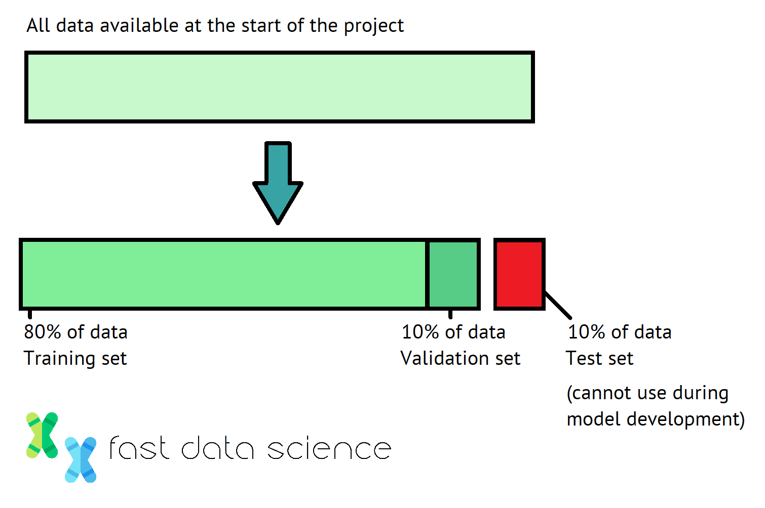
The 80-10-10 percent split commonly used for training, validation, and test data in data science.
We can use the training set in any way we like. For example, you can experiment with 1001 different models, from convolutional neural networks to LSTMs, to see which design seems to be working. You can peek at the training set to try to understand which examples your model gets wrong - for example, does it struggle with dark images, or upside-down dogs and cats?
The validation set should be used more rigorously. While we are training each model, we should monitor the performance on the validation set. We can adjust hyperparameters such as the learning rate, to see if this improves the model performance on the validation set. But we shouldn’t look into the details of where the model is going wrong.
Note that if we didn’t have a validation set, then there would be a risk of the model over-fitting on the training set. In fact, if you use the validation set too many times, it’s also possible to overfit your model to the validation set. So some researchers keep a reserve of spare validation sets to avoid this problem - of course, this is only an option if you have lots and lots of data.
Finally, the test set should be used only once: when we are finished with all training and are ready to deploy or submit the model. If your model is deployed in the wild, for example, to predict customer behaviour, then your test set is how real customers behave in the future.
One useful technique is cross-validation, where the training data and validation data are rotated and each instance gets used at least once as both training and test data. Cross-validation is useful because it lets us see how well a model will generalise to new data.
Word vector embeddings are a technique used in natural language processing, where words are mapped to vectors of real numbers. For example:
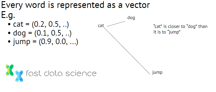
Some examples of what word vector embeddings could look like. Another classic example is ‘man’ close to ‘woman’ and ‘king’ close to ‘queen’, so you can even subtract vectors to do ‘king’ + ‘woman’ - ‘man’ = ‘queen’.
Often a large space is used, such as the 300-dimensional vector space used in word2vec.
There is a semantic similarity between words that are close together in the vector space. Below is a word2vec embedding which I trained on a set of job descriptions.
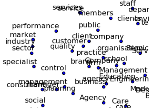
A word vector embedding trained on a dataset of text job descriptions. Note how market, industry and sector are all close together. This is a form of unsupervised learning.
The advantage of using word vector embeddings is that words in natural language can be fed into a neural network, allowing us to use deep learning to process what is fundamentally a kind of discrete data.
Explainable AI is a set of techniques for analysing and picking apart machine learning models. Some deep learning models have millions of parameters and it’s not possible for a human to comprehend what they’re all doing. With explainable AI, we introduce small perturbations in the input to a model and observe how they affect the model’s output. By doing this many times, it’s possible to gain an understanding of why a model is taking certain decisions.
Explainable AI is likely to become more important as AI regulation begins to require explanations for algorithmic decisions.
Here’s a short video we’ve made at Fast Data Science about explainable AI.
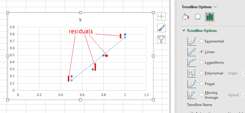
This formula is at the root of linear regression, and by extension, neural networks and much of data science. Have you ever wondered how Microsoft Excel manages to fit a straight line to a set of scattered points?
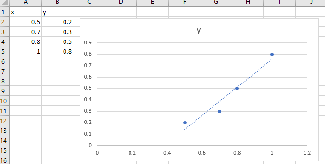
The answer is, by minimising the total loss function, ½(y - ŷ)² for all data points:

Let’s imagine our dataset is a series of points, x and y:
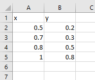
We want to train a model to fit a line

If the points don’t lie exactly on a straight line, then the error at each point will be

This is called the residual.
How to get the residual as small as possible? The maths is simpler if we try to minimise the square of the residual:

To do this, we stick ½ in front to make the result prettier, and take the sum of the residuals of all data points. We call this the loss function:

Now, when Excel has found a good fit, the loss function will be small. This happens when the gradient of the loss function equals zero. It’s possible to choose the correct values of m and c to get the loss function to the lowest possible value. This is what Excel does under the cover: it’s minimising the distance from each point in the data, to the line of best fit.
Now, here’s where we get to demystify AI and data science.
What’s a deep neural network? It’s only a series of Excel-like linear regression models, glued together with activation layers (such as the sigmoid curve). To get the lowest value of the loss function, one more bit of secret sauce is needed: the backpropagation algorithm. Read more about this in my post on how neural networks learn.
So when companies selling AI solutions talk about how ‘intelligent’ their neural networks are, and how they’ve made an AI that can write screenplays better than a human, or paint better than Picasso, this is just marketing hype. Really what these companies have is this:
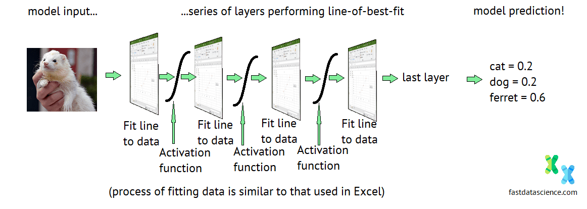
Pseudo-diagram of a neural network made up of Excel representing the ‘fit a line to data’ action.
Although I don’t want to downplay some people’s doomsday fears about a malevolent AI taking over the world, it seems to me that the most cutting-edge AIs today are the same kettle of fish as the basic Excel line-fitting function… just a few clever tricks thrown in.
That said, this year alone has shown us how suddenly catastrophes can appear, so I might be eating my words in 2021!
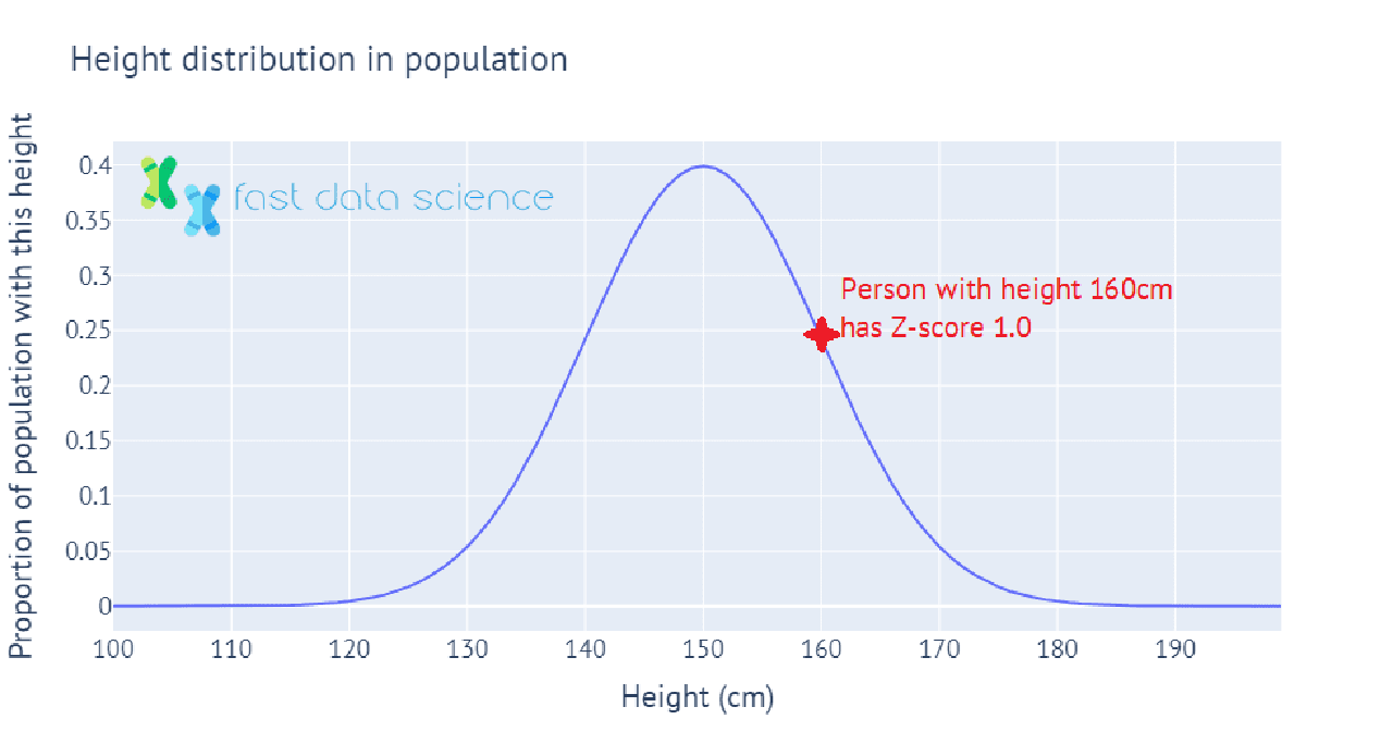
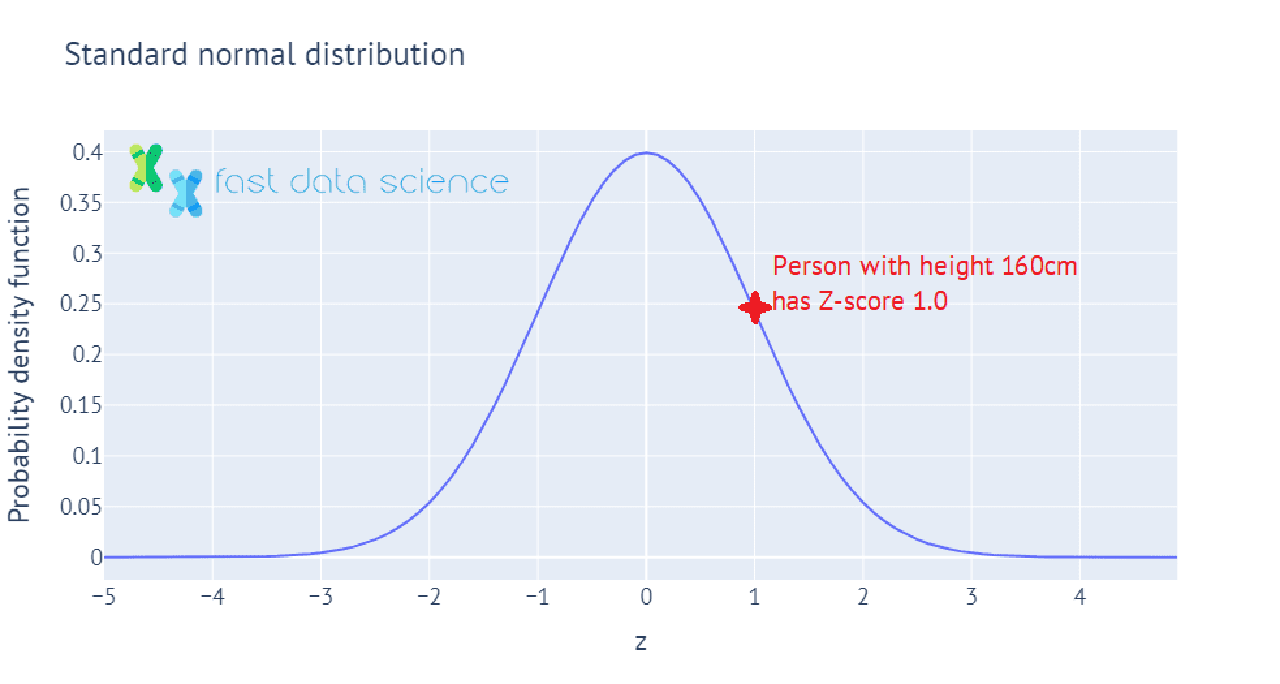
The Z-score, or standard score, is a value which tells you how many standard deviations above or below the mean a measurement lies. For example, if the population of a country has mean height 150 cm, with standard deviation 10 cm, then a person with height 150 cm would have Z-score = 0, and a person with height 160 cm would have Z-score 1.

Here’s an interactive illustration of how heights in the population can be mapped to Z-scores, showing how we calculate the Z-score for a person whose height is one standard deviation above the mean height in the population:
In statistics in practice, we often have only a sample of data, such as 100 people whose heights we have measured. In this case, we wouldn’t know the mean and standard deviation of the population’s height, so we use the mean and standard deviation of the sample of 100 instead. This value is called the t-statistic, and we can use it to perform many statistical tests, such as to test the hypothesis that the mean height of males in the population is significantly different from the mean height of females in the population.
Values such as the Z-score and t-statistic are used often by statisticians, but in machine learning and data science problems they rarely appear, since many machine learning and data science applications in industry are concerned with making predictions of e.g. customer behaviour, machine failure, vehicle loading, and the like, rather than c. However, hypothesis testing is widely used in fields such as pharmaceuticals, where for example a company might require a new drug to be effective to within 5% confidence level.
Unleash the potential of your NLP projects with the right talent. Post your job with us and attract candidates who are as passionate about natural language processing.
Hire NLP Experts
Unlock your business potential with expert AI consulting services from Fast Data Science. Discover strategies to accelerate growth and outperform competitors.

Financial advisors, like lawyers, are regulated in the UK. All financial advisors should be registered with the Financial Conduct Authority (FCA) and must have certain qualifications and have signed up to a code of ethics. UK financial advisors must also complete professional training every year.
What we can do for you