I’m introducing a Python library I’ve written, called faststylometry, which allows you to compare authors of texts by their writing style. The science of comparing authors’ fingerprints in this way is called forensic stylometry.
You will need a basic knowledge of Python to run this tutorial.
The faststylometry library uses the Burrows’ Delta algorithm, a well-known stylometric technique. The library can also calculate the probability that two books were by the same author.
I wrote this library to improve my understanding, and also because the existing libraries I could find were focused around generating graphs but did not go as far as calculating probabilities.
Here I am giving a walkthrough of how to conduct a basic stylometry analysis using the faststylometry library. We will test the Burrows’ Delta code on two “unknown” texts: Sense and Sensibility by Jane Austen, and Villette by Charlotte Brontë. Both authors are in our training corpus.
The Burrows’ delta is a statistic which expresses the distance between two authors’ writing styles. A high number like 3 implies that the two authors are very dissimilar, whereas a low number like 0.2 would imply that two books are very likely to be by the same author. Here is a link to a useful explanation of the maths and thinking behind Burrows’ Delta and how it works.
The Burrows’ delta is calculated by comparing the relative frequencies of function words such as “inside”, “and”, etc, in the two texts, taking into account their natural variation between authors.
If you’re using Python, you can install the library with the following command:
pip install faststylometry
The Jupyter notebook for this walkthrough is here.
Burrows Delta walkthrough in Jupyter Notebook
First, we start up Python. First we need to import the stylometry library:
from faststylometry import Corpus
from faststylometry import load_corpus_from_folder
from faststylometry import tokenise_remove_pronouns_en
from faststylometry import calculate_burrows_delta
from faststylometry import predict_proba, calibrate
The library depends on NLTK (the Natural Language Toolkit), so the first time that you are using it, you may need to run the following commands in your Python environment if you want to use the inbuilt tokeniser:
import nltk
nltk.download("punkt")
I have provided some test data for you to play with the library, which you can download from the project Github here. It’s a selection of classic literature from Project Gutenberg, such as Jane Austen and Charles Dickens. Due to copyright, I cannot provide more modern books, but you can always obtain them elsewhere.
If you are using Git, you can download the sample texts with this command:
git clone https://github.com/fastdatascience/faststylometry
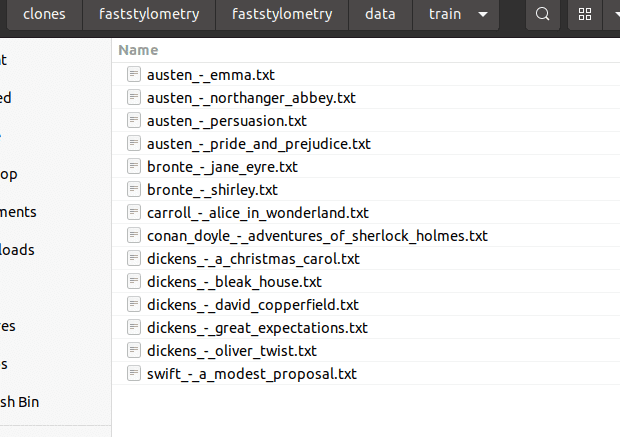
Make sure the book texts are in the folder faststylometry/data/train on your computer, and each file is named “author name”_-_“book title”.txt, for example:
You can now load the books into the library, and tokenise them using English rules:
train_corpus = load_corpus_from_folder("faststylometry/data/train")
train_corpus.tokenise(tokenise_remove_pronouns_en)
Alternatively, you can add books to your corpus using the following process:
corpus = Corpus()
corpus.add_book("Jane Austen", "Pride and Prejudice", [whole book text])
I have also provided some “unknown” books for us to test the performance of the algorithm. Imagine we have come across a work for which the author is unknown. The books I’ve included are Sense and Sensibility, written by Jane Austen (but marked as “janedoe”), and Villette, written by Charlotte Brontë, which I have marked as “currerbell”, Brontë’s real pseudonym. They are in the folder faststylometry/data/test.
 test texts](https://fastdatascience.com/images/forensic_stylometry_test_texts-min.png)
Here is the code to load the unknown documents into a new corpus, and tokenise it so that it is ready for analysis:
# Load Sense and Sensibility, written by Jane Austen (marked as "janedoe")
# and Villette, written by Charlotte Brontë (marked as "currerbell", Brontë's real pseudonym)
test_corpus = load_corpus_from_folder("faststylometry/data/test", pattern=None)
# You can set pattern to a string value to just load a subset of the corpus.
test_corpus.tokenise(tokenise_remove_pronouns_en)
Fast Data Science - London
Now we have a training corpus consisting of known authors, and a test corpus containing two “unknown” authors. The library will give us the Burrows’ Delta statistic as a matrix (Pandas dataframe) for both unknown texts (x-axis) vs all known authors (y-axis):
calculate_burrows_delta(train_corpus, test_corpus, vocab_size = 50)
We can see that the lowest values in each column, so the most likely candidates, are Brontë and Austen – who are indeed the true authors of Villette and Sense and Sensibility.
| author | currerbell – villette | janedoe – sense_and_sensibility |
|---|---|---|
| austen | 0.997936 | 0.444582 |
| bronte | 0.521358 | 0.93316 |
| carroll | 1.116466 | 1.433247 |
| conan_doyle | 0.867025 | 1.094766 |
| dickens | 0.800223 | 1.050542 |
| swift | 1.480868 | 1.565499 |
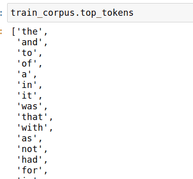
It’s possible to take a peek and see which tokens are being used for the stylometric analysis:
Now the Burrows’ delta statistic above can be a little hard to interpret, ,and sometimes what we would like would be a probability value. How likely is Jane Austen to be the author of Sense and Sensibility?
We can do this by calibrating the model. The model looks at the Burrows’ delta values between known authors, works out what are the commonest values indicating same authorship:
calibrate(train_corpus)
After calling the calibrate method, we can now ask the model to give us the probabilities corresponding to the delta values in the above table:
predict_proba(train_corpus, test_corpus)
You can see that we now have a 76% probability that Villette was written by Charlotte Brontë.
| author | currerbell – villette | janedoe – sense_and_sensibility |
|---|---|---|
| austen | 0.324233 | 0.808401 |
| bronte | 0.757315 | 0.382278 |
| carroll | 0.231463 | 0.079831 |
| conan_doyle | 0.445207 | 0.246974 |
| dickens | 0.510598 | 0.280685 |
| swift | 0.067123 | 0.049068 |
As an aside: by default the library uses Scikit Learn’s Logistic Regression to calculate the calibration curve of the model. Alternatively, we could tell it which model to use by supplying an argument to the calibrate method:

We can plot the calibration curve for a range of delta values:
import numpy as np
import matplotlib.pyplot as plt
x_values = np.arange(0, 3, 0.1)

plt.plot(x_values, train_corpus.probability_model.predict_proba(np.reshape(x_values, (-1, 1)))[:,1])
plt.xlabel("Burrows delta")
plt.ylabel("Probability of same author")
plt.title("Calibration curve of the Burrows Delta probability model\nUsing Logistic Regression with correction for class imbalance")
We can see that a value of 0 for delta would correspond to a near certainty that two books are by the same author, while a value of 2 corresponds to a near certainty that they are by different authors.
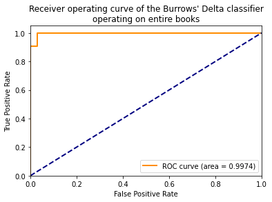
The ROC curve and the AUC metric are useful ways of measuring the performance of a classifier.
The Burrows’ Delta method, when used as a two-class text classifier (different author vs. same author), has an incredibly easy task, because it has learnt from entire books. So we would expect the classifier to perform very well.
We can perform the ROC evaluation using cross-validation. The calibration code above has taken every book out of the training corpus in turn, trained a Burrows model on the remainder, and tested it against the withheld book. We take the probability scores resulting from this, and calculate the ROC curve.
An AUC score of 0.5 means that a classifier is performing badly, and 1.0 is a perfect score. Let’s see how well our model performs.
First, let’s get the ground truths ( False = different author, True = same author) and Burrows’ delta values for all the comparisons that can be made within the training corpus:
ground_truths, deltas = get_calibration_curve(train_corpus)

We get the probabilities of each comparison the model has made by putting the Burrows’ delta values back through the trained Scikit-Learn model:
probabilities = train_corpus.probability_model.predict_proba(np.reshape(deltas, (-1, 1)))[:,1]
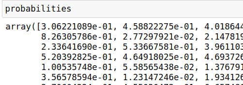
We can put the probabilities and ground truths into Scikit-Learn to calculate the ROC curve:
from sklearn.metrics import roc_curve, auc
fpr, tpr, thresholds = roc_curve(ground_truths, probabilities)
We can now calculate the AUC score. If our model is good at identifying authorship, we should see a number close to 1.0.
roc_auc = auc(fpr, tpr)
Finally, we can plot the ROC curve:
plt.figure()
plt.plot(fpr, tpr, color='darkorange',
         lw=lw, label='ROC curve (area = %0.4f)' % roc_auc)
plt.plot([0, 1], [0, 1], color='navy', lw=2, linestyle='--')
plt.xlim([0.0, 1.0])
plt.ylim([0.0, 1.05])
plt.xlabel('False Positive Rate')
plt.ylabel('True Positive Rate')
plt.title('Receiver operating curve of the Burrows\' Delta classifier\noperating on entire books')
plt.legend(loc="lower right")
plt.show()
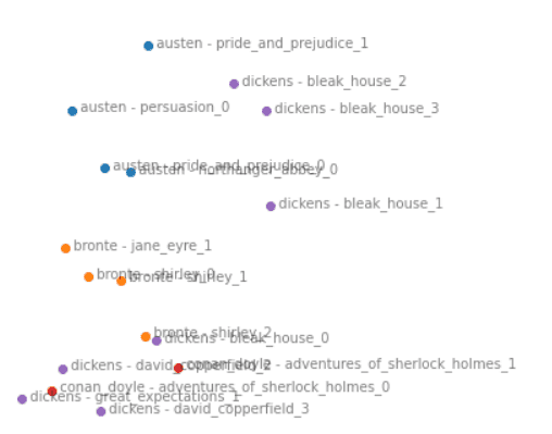
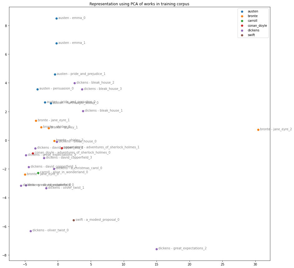
We can also visualise the stylistic similarities between the books in the training corpus, by calculating their differences and using Principal Component Analysis (PCA) to display them in 2D space.
For this, we need to use the Python machine learning library Scikit-Learn.
from sklearn.decomposition import PCA
import re
import pandas as pd
We can re-load the training corpus, and take segments of 80,000 words, so that we can include different sections of each book in our analysis.
# Reload the training corpus as the "test corpus", re-tokenise it, and segment it this time
test_corpus = load_corpus_from_folder("faststylometry/data/train")
test_corpus.tokenise(tokenise_remove_pronouns_en)
split_test_corpus = test_corpus.split(80000)
Now we calculate the Burrows’ delta statistic on the book segments:
df_delta = calculate_burrows_delta(train_corpus, split_test_corpus)
We are interested in the array of z-scores
df_z_scores = split_test_corpus.df_author_z_scores
The above array is too big to display directly, so we need to reduce it to two-dimensional space to show it in a graph. We can do this using Scikit-Learn’s principal component analysis model, setting it to 2 dimensions:
pca_model = PCA(n_components=2)
pca_matrix = pca_model.fit_transform(df_z_scores)
It would be nice to plot the book sections on a graph, using the same colour for every book by the same author. Since the Z-scores matrix is indexed by author and book name, we can use a regex to take everything before the first hyphen. This gives us the plain author name with the book title removed:
authors = df_z_scores.index.map([lambda](https://aws.amazon.com/lambda) x : re.sub(" - .+", "", x))

We can join the PCA-derived coordinates and the author names together into one dataframe:
df_pca_by_author = pd.DataFrame(pca_matrix)
df_pca_by_author["author"] = authors
Now we can plot the individual books on a single graph:
plt.figure(figsize=(15,15))
for author, pca_coordinates in df_pca_by_author.groupby("author"):
    plt.scatter(*zip(*pca_coordinates.drop("author", axis=1).to_numpy()), label=author)
for i in range(len(pca_matrix)):
    plt.text(pca_matrix[i][0], pca_matrix[i][1],"  " + df_z_scores.index[i], alpha=0.5)
plt.legend()
plt.title("Representation using PCA of works in training corpus")
The code for the ROC/AUC means that we can try out different parameters, changing the vocabulary size, document length, or preprocessing steps, to see how this affects the performance of the Burrows’ delta method.
I would be interested to find out how the delta performs on other languages, and if it would be beneficial to perform morphological analysis as a preprocessing step in the case of inflected languages. For example, in the Turkish word “teyzemle” (with my aunt), should this be treated as teyze+m+le, with the two suffixes input separately?
You can try this kind of experiment by replacing the function tokenise_remove_pronouns_en with a tokenisation function of your choice. The only constraint is that it must convert a string to a list of strings.
If you are undertaking research in AI, NLP, or other areas, and are publishing your findings, I would be grateful if you could please cite the project.
Wood, T.A., Fast Stylometry [Computer software] (1.0.4). Data Science Ltd. DOI: 10.5281/zenodo.11096941, accessed at https://fastdatascience.com/natural-language-processing/fast-stylometry-python-library/, Fast Data Science (2024)
A BibTeX entry for LaTeX users is:
@software{faststylometry,
    author = {Wood, T.A.},
    title  = {Fast Stylometry (Computer software), Version 1.0.4},
    year   = {2024},
    url = {https://fastdatascience.com/natural-language-processing/fast-stylometry-python-library/},
    doi = {10.5281/zenodo.11096941},
}
Thankfully, a number of people and organisations around the world have been using the Fast Stylometry library and have cited us.
Yong-Bin Kang at the Australian Research Council (ARC) Centre of Excellence for Automated Decision-Making and Society used the tool for analysing content on mental health forums:
Rebecca Hicke and David Mimno at Cornell University used Fast Stylometry for author attribution in early modern English drama:
You can try out the free open source library that we have developed, Fast Stylometry (https://github.com/fastdatascience/faststylometry). This will output the probability that an unknown document is written by a particular author.
However, please check how long the document is? Are we talking complete books, or just short letters?
Often, stylometry is only effective if you have long documents, i.e. at least a chapter length, to compare. Ideally your documents that you are comparing are of the same type of document, e.g. novels vs novels, speeches vs speeches. Trying to compare across document types can be difficult.
As the field moves on, large language models may reduce the amount of text needed to reach a conclusion. However, a single page, or short email, is usually far too short to be able to reach a conclusion on authorship with any certainty. Please note that high-profile stylometry “detective work”, like the identification of JK Rowling as the author of The Cuckoo’s Calling, involved entire novels. If you only have a couple of pages of text, we are unlikely to be able to do anything. However, feel free to get in touch with Fast Data Science as it may still be worth us taking a look.
It is difficult to prove authorship one way or the other, however, the technology you are referring to is forensic stylometry. We have built an open source library which can run stylometry analyses. Ideally you need documents that are at least the length of a book chapter. Emails and letters are generally too short. A stylometry analysis can give you a percentage likelihood of a given person being the author of a document, provided we have enough documents from that person. The algorithm commonly used for this is called Burrows’ Delta and it has been around for quite some time, predating LLMs.
If you have documents with known authors, this is a good start. The Fast Stylometry Python library allows you to calculate a “Burrows’ Delta” score, which measures the linguistic distance between an anonymous text and a corpus of known works by analysing frequent word patterns and deducing a “fingerprint” of each author.
With the documents you have, you can work out a typical Burrows’ Delta for two documents from different authors vs the typical Delta for two documents from the same author.
If your documents are short, you’re likely to see a lot of overlap as you need quite some length of document, typically a book chapter’s length, before you would have enough data to draw any conclusions. This is especially true if you want something that will stand up as evidence in a civil or criminal case. Please get in touch with Fast Data Science to discuss your needs in more detail.
Looking for experts in Natural Language Processing? Post your job openings with us and find your ideal candidate today!
Post a Job
Unlock your business potential with expert AI consulting services from Fast Data Science. Discover strategies to accelerate growth and outperform competitors.

Financial advisors, like lawyers, are regulated in the UK. All financial advisors should be registered with the Financial Conduct Authority (FCA) and must have certain qualifications and have signed up to a code of ethics. UK financial advisors must also complete professional training every year.
What we can do for you